3 Mining transactional data

Mining transactional data—frequent item-sets chapter 6 

Frequent itemsets: sup(I) >= s

Support of I:

sup(I) = # baskets that contains all items in I

Support ratio = sup(I)/n

n = # baskets

Maximally frequent: 

I is frequent, none of I’s supersets is frequent

Applications: 

1. Baskets—transactions// documents

2. Items—products// words

3. Frequent item sets: products frequently bought together// Words that occur together frequently in many documents

Association rules:

I —>j ( I: a set of items, J: an item )

I: a set of items, j: an item

If all of items in I appear in some baskets, then j likely appears in that baskets too

Confidence( I->j )= sup(I U{j})/sup(I)

Finding rules with high confidence:

I —>j: both of sup(I U{j}) and sup(I) should be high 

1. For frequent item sets
2. For each of them j, determine if J-{j}—>j has high confidence  for j belongs to J 

Interest of rules

Interest(I->j) = conf(I->j)-sup_ratio({j})

Apriori  algorithms:

Make 2 passes

1. Find frequent 1-itemsets
2. Find frequent pairs only pairs of frequent items are considered 

1 pass

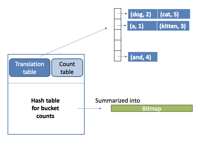
1. Data structure: 

1) Translation table T: item names => integers 

Idea: representing items using integers, hash table.

a. for each item x in the basket file 

b. hash x to a bucket in the table, initialize sequence # s = 1

c. if x is not yet in the bucket, assign s to x, record x and its number in the bucket, increment s 

2) Count table C1: i-th element storing count of i-th item, initially all counts = 0 

Idea: Triangular-matrix = Stored as an array with n(n-1)/2 counts

         Triples = (i, j, count) 

1. Read baskets
2. for each baskets:  1) translate each of its item to an int, i    2)Increment the count of the i th element in C1
3. Return items with sufficient support 

Count table --> Frequent items table F 

key 1-m = index range of m frequent items

value 1~n = old item index 

2 pass: 

finding frequent pairs 

for each basket:

a. find frequent items using F

b. generate pairs of them 

c. count each pair

2+ passes 

Pass k, 2 sets are used: 

1. Ck--candidate k-itemsets + Lk--frequent k-itemsets

2. For k-itemsets, use k+1-tuple (i1, i2, ..., ik, count) 

k = 1

C1 = all items 

Ck filter: remove the infrequent --->Lk need 1 pass through all baskets 

Apriori

子集包含关系：形成一个k+1 candidate itemsets Ck+1, 它的k 子集必须都是frequent k-itemsets

SON alg:

 Map reduce for finding frequent item sets

1. divide basket file into chunks, fraction p 

2. treat chunk as sample 

3. run discovery alg on the sample --support threshold = p*s 

4. collect frequent itemset from chunks. form candidate item sets

5. 2nd pass through baskets: collect counts for candidates. return frequent ones

Properties:

• a global frequent itemset may not always local frequent (all chunks), but at least in 1 chunk, it is frequent 
• false negative: LOCAL yes GLOBAL no. local infrequent can be frequent, global infrequent cannot be frequent 
• false positive:  LOCAL yes GLOBAL no. local frequent can be infrequent in some other chunks, but global cannot 

Apriori with Son framework  

Two phases

• Phase 1: Find candidate itemsets (local frequent)

找出各个sample中所有 可能global frequent的 local frequent itemsets

a. Map:
– Input: a chunk of basket file
– Output: (F, 1)'s, where F is a local frequent itemset
e.g:

Chunk 1: 
– (1, 1), (2, 1), (3, 1), (4, 1)
– ((1, 2), 1), ((1,3), 1), ..., ((3,4), 1)
– ((1,2,3), 1), ((1,3,4), 1), ((2,3,4), 1)
Chunk 2: 
– (1, 1), (2, 1), (3, 1), (4, 1), (5, 1)
– ((1, 2), 1), ((1,3), 1), ((1,4), 1), ((2,3),1), ..., ((3,5), 1) 
– ((1,2,3), 1), ((1,2,4), 1), ((2,3,5), 1) 

b. Reduce:
– Input: (F, a list of 1's) -- count-filter
– Output: (F, 1)-- local frequent 
e.g.
 (1, 1), (2, 1), (3, 1), (4, 1), (5, 1)

((1, 2), 1), ((1,3), 1), ..., ((3,4), 1), ((3,5), 1) ((1,2,3), 1), ((1,2,4), 1), ((1,3,4), 1), ((2,3,4), 1),
((2,3,5), 1) 

• Phase 2:Collect counts & find global frequent itemsets 

对phase1得到的local frequent itemsets进行global count，全局筛选

a. Map:

– Input: all candidate itemsets and a subset of baskets

– Output: (C, v)'s, where C is a candidate itemset, v is C's count in the subset

chunk1:
– (1, 4), (2, 4), (3, 4), (4, 3), (5, 1) – ((1, 2), 3), ((1,3), 4), ...
–...
chunk2:
– (1, 4), (2, 5), (3, 3), (4, 2), (5, 2) – ((1, 2), 4), ((1,3), 2), ...

b. Reduce:
– Input: (C, list of v's)

(1, [4,4]), ...

– Output: (C, sum of v's) if global frequent 

(1, 8), (2, 9), (3, 7), (4, 5), ((1,2), 7), ...

Apriori with Son framework ALG OPTIMIZATION 

The main time reduction is in my "candidate generation, L to C" step in apriori,

To be a candidate item set, all of its immediate subsets must be in  the previous frequent list.

there may be multiple methods to realize filter, here share 2 methods:

1) Logical method to remove "ineligible combined set" 

python code:

if [i for i in combinations(j,k-1) if i not in Li_1] == []:

2) Mathematical Inference to remove "ineligible combined set

we count the # of  generated larger item-set from the frequent item-sets and use "generated item-set: count" to build a dictionary.

From a mathematical perspective, we can assume a item-set is candidate, which means that all of its immediate subsets are in the frequent list.

so how many immediate subsets for a candidate item-set of size n?

C(n,n-1)

it means that a item-set must have C(n,n-1) sons in frequent item-sets, then it can be a candidate to be count in the future 

e.g.

if the member of frequent list is composed by 2 elements, like (1,2) (3,2) (1,3)

then the generated item-set size is 3, like (1,2,3)

if (1,2) (3,2) (1,3) is frequent, then (1,2,3) can be a candidate

Handling larger datasets in memory 

PCY 

leverage unused memory in pass 1

discover some of infrequent pairs

reduce candidates pairs in pass 2 (C2)

Memory requirement 

T hash table of item names plus counts n, e.g.24n 

C Count table: 4n bytes

Idea

create frequent bucket in pass 1--> hash every pair of items to the bucket 

2nd pass:

– Generate candidate pair (i, j) only when it hashes to a frequent bucket >= s 

– i and j are both in L1 

Frequent buckets 
1. no false negatives, but it may have false positives
e.g. If a pair hashes to a frequent bucket, it may still be infrequent (why?) 

2. False positive rate  = % of frequent buckets p = bf/b 

bf ≤ total # of pairs / 𝑠 

p ≤ total # of pairs / b*s (= avg # 𝑜f pairs per bucket / s )

Multistage 

similar to PCY, but use extra passes to further reduce size of C2

Multihash

Toivonen: 

After determining the frequent itemsets in the sample, the algorithm builds the negative borders from the frequent itemsets. Then it considers the entire data to calculate the frequency of the negative borders. If any of the negative borders are frequent, we run the sampling again with a new random sample as we may have frequent itemsets not covered in our initial sample. Else the obtained frequent itemsets from the sample contain the final result.

Minimally infrequent 

•  maximally frequent, if
– I is frequent, and if add any item to I, it will become infrequent 

• minimally infrequent, if 

– I is infrequent, and if remove any item from I, it will become frequent 

– (I is in "negative border" in Toivonen) 

• Every infrequent itemset is 

– either minimally infrequent or a superset of some minimally infrequent itemset 

• If I is not minimally infrequent, one of its subsets, say Y, must be infrequent 
• If Y is not minimally infrequent, continue to find its infrequent subset
• The above process stops at some 1-itemset X 
• X is surely minimally infrequent 

Toivonen's algorithm steps

1. Start with steps similar to that in SAMPLE alg.
 –  a sample of baskets– Find candidate frequent itemsets in the sample 

2. Construct negative borders 
– Itemsets infrequent in the sample 
– But all immediate subsets (i.e., 1 item less) are frequent in the sample

3. Check if item-sets frequent locally & ones in the negative border are GLOBALLY frequent– Need to make 1 pass through the data set 

4. If ALL itemsets in the negative border are IN-frequent in the entire data set 
– Itemsets frequent LOCALLY & also frequent GLOBALLY are the only frequent itemsets 

5. If some itemsets in the negative border are frequent in the entire data set, 
–  There may be other frequent items 
–  No answers are given in this case 
–  May re-execute the algorithm with a new sample 

WHY？

Negative border is a set of minimally infrequent itemsets in the sample 

– All other infrequent itemsets are supersets of itemsets in the negative border 

⇒If none of itemsets in negative border is global frequent, none of its supersets can be 

(and we know its supersets include all other infrequent itemsets) 

May use .9ps / .8ps (instead ps) for sample 

– s = support threshold for entire dataset 

– p = sampling rate 

This in effect pushes down the border, reduces the chance of finding global frequent itemsets in negative border (i.e., false negatives) 

– Hence the chance of having to rerun algorithm 

– Cost: more false positives LACALLY